Contents
CE gap between pass 16 and recurrence across both checkpoints.
Best final recurrent CE in this set: s9e11.
s9e12’s final top-16 FFN output subspace overlap.
1What this set compares#
Each model has an eight-layer encoder and an eight-layer decoder. Jacobi evaluation runs the encoder once, then reuses the decoder for successive passes over the sequence. Recurrent evaluation instead runs the decoder once per token, carrying the previous token’s compacted bank and causal attention state forward.
- Stack
- 8 layers · width 1,024 · FFNs 3,072
- Token attention
- 8 query heads · 2 K/V heads
- Carried state
- One 1,024-wide bank
- Engram
- After layer 2’s attention and FFN
- Batch
- 128 sequences × 4,096 positions
- Objective
- Cross entropy only; no MSE term
The compactor reads 17 fresh sources: the 16 attention/FFN outputs and the Engram output. It RMS-normalizes each source, applies its receiving-token mask, gathers, then projects to the outgoing bank. The ordinary embedding and incoming bank are outside this compaction pool.
Each update uses six microbatches with pass losses [.3, .7], and two with
[0, 0, .5, .5]. Gradients flow through all passes. The decoder’s active shape is the same across this
set; tying weights changes the number of unique parameters.
| Run | Attention | Feed-forward layers |
|---|---|---|
s9e2 | Independent attention | Independent FFNs |
s9e5 | Shared attention | Shared FFNs + compaction masks |
s9e6 | Summed attention matrices | Summed FFNs |
s9e7 | Shared attention | Summed FFNs |
s9e8 | Shared attention | Independent FFNs |
s9e9 | Shared K/V; separate Q/O | Independent FFNs |
s9e10 | Shared K/V/O; separate Q | Independent FFNs |
s9e11 | Shared K/V/O; summed Q | Summed FFNs |
s9e12 | Shared K/V/O; annealed summed Q | Annealed summed FFNs |
Shared means the same parameters are used by encoder and decoder. Summed means the encoder uses while the decoder uses . The annealed version replaces the sum by and gradually reduces .
The attention labels summarize the main sharing choices. K/V sharing also includes K normalization and the K/V/X convolutions and XSA parameters. Ordinary layer and Engram-context residual readers remain separate; the output head’s current-history query is shared. s9e5 additionally shares compaction masks, so it changes more than the dense matrices alone.
2Early passes and recurrent quality#
The ranking depends on which computation we score. At the final checkpoint, s9e2 has the best pass-2 CE (2.2985), but the weakest recurrent CE in this set (2.3254). s9e11 has the best recurrent score, 2.3072. The encoder-assisted early computation and repeated decoder computation are producing different quality rankings.
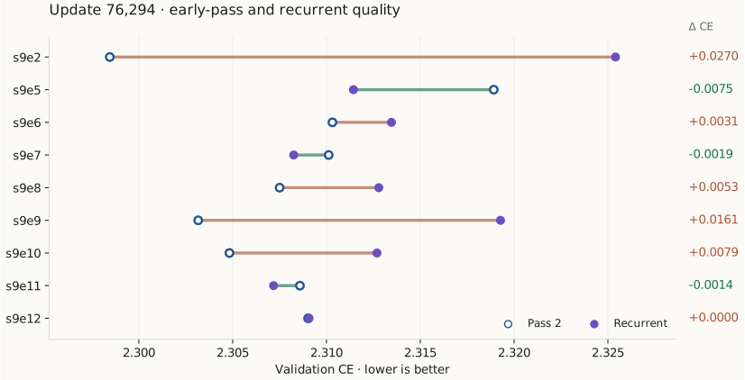
| Run | Pass 2 | Pass 4 | Pass 16 | Recurrent | Δ vs pass 2 |
|---|---|---|---|---|---|
s9e2 | 2.298454 | 2.309114 | 2.325066 | 2.325405 | +0.026951 |
s9e5 | 2.318916 | 2.311472 | 2.311407 | 2.311438 | -0.007478 |
s9e6 | 2.310318 | 2.309671 | 2.313451 | 2.313464 | +0.003146 |
s9e7 | 2.310119 | 2.307573 | 2.308240 | 2.308254 | -0.001865 |
s9e8 | 2.307504 | 2.309560 | 2.312763 | 2.312790 | +0.005286 |
s9e9 | 2.303166 | 2.310644 | 2.319216 | 2.319278 | +0.016112 |
s9e10 | 2.304830 | 2.307806 | 2.312653 | 2.312692 | +0.007862 |
s9e11 | 2.308587 | 2.306375 | 2.307167 | 2.307180 | -0.001407 |
s9e12 | 2.309023 | 2.307665 | 2.309041 | 2.309071 | +0.000048 |
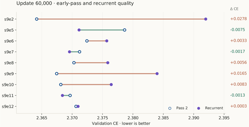
| Run | Pass 2 | Pass 4 | Pass 16 | Recurrent | Δ vs pass 2 |
|---|---|---|---|---|---|
s9e2 | 2.364174 | 2.376030 | 2.391740 | 2.391979 | +0.027805 |
s9e5 | 2.378634 | 2.371163 | 2.371122 | 2.371141 | -0.007493 |
s9e6 | 2.372434 | 2.372142 | 2.375686 | 2.375701 | +0.003266 |
s9e7 | 2.371223 | 2.368888 | 2.369563 | 2.369569 | -0.001654 |
s9e8 | 2.370301 | 2.372736 | 2.375845 | 2.375867 | +0.005566 |
s9e9 | 2.367458 | 2.375721 | 2.383921 | 2.383978 | +0.016519 |
s9e10 | 2.368139 | 2.371766 | 2.376413 | 2.376435 | +0.008297 |
s9e11 | 2.369667 | 2.367623 | 2.368388 | 2.368407 | -0.001260 |
s9e12 | 2.370640 | 2.369612 | 2.370955 | 2.370979 | +0.000338 |
Pass 16 is already a close proxy for recurrence here. Across all nine runs at both checkpoints, the absolute gap is at most 0.00034 nats/token. The larger distinction is between early passes and that endpoint. The small remaining differences can include BF16 rounding from different matrix shapes as well as incomplete refinement; they should not be read as a large stability problem.
At the end, s9e5 improves from 2.3189 at pass 2 to 2.3114 in recurrence. s9e7 and s9e11 also retain a small gain over pass 2, although their best measured score is at pass 4. Other models lose some of the encoder-assisted advantage. More iterations therefore need to be judged by their final prediction quality, not only by whether the states converge.
3The useful comparisons#
| Comparison | Change | Recurrent Δ CE |
|---|---|---|
s9e8 vs s9e2 | Share attention; keep FFNs independent | -0.01262 |
s9e7 vs s9e8 | Use summed FFNs under shared attention | -0.00454 |
s9e10 vs s9e9 | Share O as well as K/V | -0.00659 |
s9e11 vs s9e10 | Add summed Q and summed FFNs | -0.00551 |
s9e12 vs s9e11 | Anneal the sum coefficient | +0.00189 |
Two comparisons look useful for the next round. Summed FFNs improve on independent FFNs when attention is shared (s9e7 versus s9e8). Sharing O also helps when K/V are already shared (s9e10 versus s9e9). The best endpoint comes from shared K/V/O with summed Q and FFNs, s9e11.
Annealing the coupling away in s9e12 does not improve the final score over s9e11 in these runs; it is higher by 0.00189 CE. That is a result to replicate before drawing a broad conclusion about annealing.
These are single runs. The s9e11/s9e10 comparison changes Q and FFNs together, so it cannot isolate which supplies the gain. The downloadable data includes paired document intervals; those intervals cover validation sampling, not variation between training seeds.
4Are the output spaces actually aligned?#
This is measured from the trained matrices, not inferred only from the sum. For each layer, take the FFN down-projection, which maps hidden features back into the 1,024-wide residual space. Compare its leading encoder and decoder output directions using the left singular vectors.
and contain orthonormal leading left singular vectors. The squared Frobenius norm is the sum of squared matrix entries. The result is the mean squared cosine of the principal angles: 0 means orthogonal subspaces; 1 means the same subspace. We average the score across the eight FFNs.
For the leading 16 directions at 60k, s9e7 has overlap 0.789, versus 0.368 for s9e8. s9e11 is at 0.794, s9e12 at 0.709, and s9e2 at 0.116. Independent isotropic 16-dimensional subspaces in 1,024 dimensions would average 0.015625. The same broad pattern holds at 8, 32 and 64 directions.
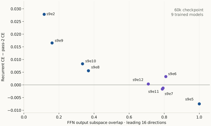
One plausible interpretation is that compatible encoder and decoder output spaces reduce the quality change when later passes rely on decoder-generated features. There is another explanation mixed into the same experiments: the summed parameterization also routes encoder gradients into decoder weights. These measurements do not separate representation compatibility from that optimization effect.
These are dominant weight directions. The top 16 carry only about 5–6% of squared weight norm, so 0.79 overlap does not mean 79% of activations or information is shared. Activation covariance has not been measured. Unlike raw weight cosine, this output-subspace comparison is unchanged by a permutation of the FFN’s hidden neurons.
The extra weights are substantial
Stored is roughly as large as , not a small correction. With the fixed sum, effective encoder FFN weights have about 1.8 times the decoder’s norm. The input norm gains are separate and can compensate, so this does not imply 1.8 times the activation magnitude.
A best rank-64 approximation to the stored FFN corrections retains only 16.2–16.9% of their squared weight norm. Rank 256 retains about 49%; roughly 720 of 1,024 possible directions are needed for 90%. That makes aggressive post-training low-rank compression an uncertain shortcut. It does not rule out training a smaller adapter from the outset.
There is also an attention-side clue: adding shared O in s9e10 coincides with stronger alignment of its untied Q matrices. Mean encoder/decoder Q cosine rises from 0.143 to 0.573, and leading-16 output-subspace overlap from about 0.116 to 0.499. This is another association worth isolating, rather than proof of a mechanism.
5Does s9e12 keep the alignment at the end?#
Yes. The top-16 overlap is 0.6979 at the final checkpoint, versus 0.7094 at 60k. The decrease is only 0.0115, and the result is similar at the other ranks.
| Leading directions | Step 60,000 | Final · 76,294 |
|---|---|---|
| 8 | 0.7016 | 0.6865 |
| 16 | 0.7094 | 0.6979 |
| 32 | 0.6945 | 0.6862 |
| 64 | 0.6933 | 0.6859 |
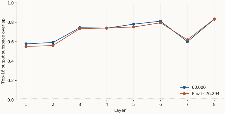
The encoder uses , while the decoder uses . As falls, the compensation update moves the removed shared contribution into , preserving the effective encoder weights across the change in . At the final checkpoint , but that does not erase the earlier training history.
Final per-layer overlap ranges from 0.55 to 0.83. The leading 16 directions contain 6.50% of encoder and 5.55% of decoder squared weight norm. The alignment is therefore persistent, but it remains a measurement of selected weight directions rather than a complete description of the representations.
6What the banks and layers are doing#
The forward magnitudes settle quickly. On the matched diagnostic panel, s9e2’s mean incoming-bank L2 norm falls from 71.36 at pass 2 to 66.72 at pass 4 and 66.65 in recurrence. Its predictions still get worse beyond pass 2. Bounded states and a good recurrent predictor are different requirements.
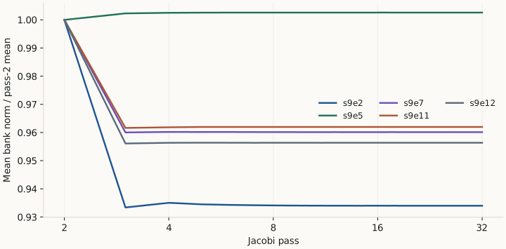
| Run | Pass-2 mean | Pass-4 mean | Recurrent mean ± SD |
|---|---|---|---|
s9e2 | 71.36 | 66.72 | 66.65 ± 21.79 |
s9e5 | 64.62 | 64.79 | 64.79 ± 18.34 |
s9e6 | 66.81 | 63.61 | 63.59 ± 20.10 |
s9e7 | 64.06 | 61.51 | 61.50 ± 20.04 |
s9e8 | 67.85 | 63.76 | 63.76 ± 21.62 |
s9e9 | 69.77 | 63.92 | 63.90 ± 21.33 |
s9e10 | 67.22 | 62.82 | 62.81 ± 20.37 |
s9e11 | 62.38 | 60.00 | 60.01 ± 18.86 |
s9e12 | 64.73 | 61.91 | 61.91 ± 19.95 |
Across all nine models, recurrent mean bank norms are 60.01–66.65, with tokenwise standard deviations 18.34–21.79. Every mean attention/FFN/Engram output norm is within 0.23% of its pass-4 counterpart. The magnitude difference is too small to be a simple explanation for the loss ordering. Directions and information content can still differ.
Memory is read most directly near the bottom
The incoming bank gets 0.52–0.81 of the first attention reader’s probability and 0.26–0.48 of the first FFN reader’s. At the final output gather it gets only 0.002–0.006. This is a consistent routing pattern across the set.
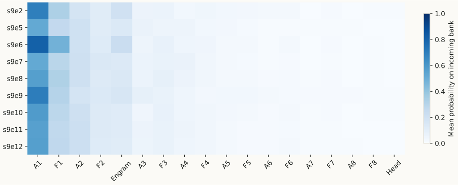
The compactor itself mixes broadly: its entropy-equivalent number of selected sources averages 14.0–15.1 out of 17. Each fresh source is normalized before masking and gathering, so a large raw layer output does not directly pass its scale into the bank.
A small direct bank weight near the top does not mean the bank is irrelevant there. Its information may already be present in earlier layer outputs. These are forward measurements; they do not establish that gradients through long recurrences are bounded.
7What seems worth testing next#
My strongest next test would isolate a shared FFN output basis: share the down-projection, while keeping the up and gate projections independent. That is a narrower intervention than summing every FFN matrix, and would help distinguish the output-space hypothesis from general weight coupling.
A second test would put more of the CE objective on later decoder states, while tracking the extra training cost. The early-pass advantage can disappear even when the forward state settles. Improving the quality of that limiting computation looks more relevant here than adding damping solely because late-pass CE is worse.
The routing pattern also motivates a controlled bank-injection ablation before reducing how much of the stack recurs. Limiting injection to lower readers might be enough, but the probability plots cannot establish that: the comparison needs a trained model and the same recurrent evaluation.
Finally, a small adapter remains worth testing as a fresh parameterization. The current corrections are large and broadly distributed across singular directions, so their existing spectra do not promise that low-rank compression will preserve quality.
8Scope, data and limits#
- Full validation: 4,800 identical documents, 4,749,346 scored next-token targets, at updates 60,000 and 76,294. CE is token weighted and unweighted by training-loss coefficients.
- Dynamics and routing: a separate matched panel of 64 documents, sampled from four length strata and capped at 1,024 positions, with 38,083 targets. Panel magnitudes and probabilities are comparable across modes and models; its CE is not substituted for the full report.
- Weight geometry: all nine 60k checkpoints, plus s9e12’s final FFN output projections. Float64 decompositions passed orthogonality and singular-relation checks.
- Limits: one trained run per architecture, no seed replications, and some comparisons change multiple components. Weight spectra are not the Jacobian of the whole recurrent transition. These results motivate specific tests rather than proving a general convergence mechanism.
This log is a dated snapshot of the current measurements. It may change as the hypotheses are tested. The earlier experiment history is in the Setting 3 worklog; the broader motivation is in the research plan.